Buckley Leverett analysis in Python

I thought it would be interesting to write some functions to perform a Buckley-Leverett analysis using python and matplotlib.

The theory

The Buckley-Leverett partial differential equation is:

As $S_w(x,t)$ we can write the total derivative as:

and, given that the fluid front is of constant saturation in the analysis, we can say:

Substituting this into the Buckley-Leverett equation, gives:

Integration of both sides over time $t=0$ to $t=t$:

gives an expression for the position of the fluid front $x_f$ at time $t$:

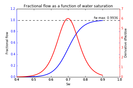
As we know that the fractional flow in the simple case of horizontal flow can be calculated as:

we can plot this, along with it’s derivative $\frac{df_w}{dS_w}$ calculated numerically:

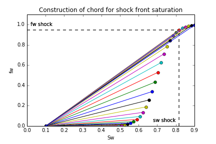
To determine the water saturation at the shock front, we can construct chords starting at the connate water saturation, working our way up the fractional flow curve until we find the maximum gradient - this point gives us the shock saturation. In this case, $S_w = 0.81$:

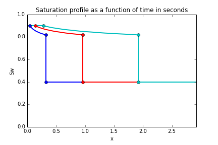
Then we can plot the saturation as a function of the position $x_f$.

The curve suggests there exists two saturation solutions at each distance step, which is not physically possible. The shock front saturation is a discontinuity, and this can be used to modify the plot above to yield a profile of the saturation behind and in front of the saturation front.

• $S_{w i}$ represents the initial water saturation, where the shock front has not yet reached
• $S_{w \ shock}$ represents the water saturation at the shock front
• $1-S_{or}$ represents the water saturation behind the shock front, after the saturation front has swept through, this location is left at the residual oil saturation, $S_{or}$ .

The code

The Buckley-Leverett class contains the relevant attributes for each instance, including the permeabiliy end points which can be used to generate the relative permeability curves using Corey type relationships.

class BuckleyLev():
    
    def __init__(self):
        self.params = {
            #non wetting phase viscosity
            "viscosity_o": 1.e-3,
            #wetting phase viscosity
            "viscosity_w": 0.5e-3,
            #initial water sat
            "initial_sw":0.4,
            #irreducable water saturation, Swirr
            "residual_w":0.1,
            #residual oil saturation, Sor
            "residual_o":0.1,
            #water rel perm at water curve end point
            "krwe":1,
            #oil rel perm at oil curve end point
            "kroe": 0.9,
            #porosity
            'poro':0.24,
            #water injection rate units m3/hr
            "inject_rate":200,
            #cross sectional area units m2
            "x-area":30
        }

Using the these instance attributes we can then add methods to the class for calculating the fractional flow:

def fractional_flow(self,sw):
    #returns the fractional flow
    
    return 1./(1.+((self.k_rn(sw)/self.k_rw(sw))*(self.params["viscosity_w"]/self.params["viscosity_o"])))

BuckleyLev.fractional_flow = fractional_flow

and for calculating the derivative numerically a finite difference approximation:

def fractional_flow_deriv(self,sw):
    #calculate derivative of fractional flow - dFw/dSw - Vsh
    
    f_deriv = (self.fractional_flow(sw+0.0001) - self.fractional_flow(sw))/0.0001
    
    return f_deriv

BuckleyLev.fractional_flow_deriv = fractional_flow_deriv

The full code is available here

By defining the attirbutes in this way, we can also visualise at the effects of evaluating the position of the shock as it progresses at different time steps, as follows:

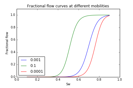
Another interesting property is the actual proerties of the fluids involved in the displacement. The mobility ratio is defined as $\frac{k_{ro}}{\mu_o}$. For a higher viscosity oil, the mobility ratio is lower. We can see the effects of this in the below figure - a more viscous oil means the water brekthrough occurs earlier.